Machine Learning - Regression explained

Regression

According to Wikipedia definition of Regression

' regression analysis is a set of statistical processes for estimating the relationships among variables. It includes many techniques for modeling and analyzing several variables, when the focus is on the relationship between a dependent variable and one or more independent variables'  

-😏'I was suppose to learn AI in simpler way' 

Hold on we moving toward learning AI only. Starting with the high school mathematics lets recall 'Sets and Function'

A function is a relation between a set of inputs and a set of permissible outputs with the property that each input is related to exactly one output

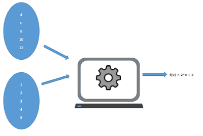
😓 QUIZ :- Can you find a relation between these two sets of data with your human intelligence?

Yes you guessed it right, Mathematically the above function is 

                         Y= f(x) = 2*x + 2

So in a world of Artificial Intelligence this mapping for the set of numbers or finding a semantic relation between numbers in form of a mathematical function is called Regression. 

-😏'But How can I make my Computer learn this function'

    

We will give both sets of data to our Computer Code that will find the suitable function for it

Plotting the X and Y values gives us the interpretation that it is a Linear Regression. So we can start off our Computer Code with a General Equation of line i.e:-

                    Y= f(x) = m*x + c

and assume any random value for slope m and intercept c. Let it be m=0 and c=1, Now
                    Y= f(x) = 0*x + 1;
                    Y= f(x) = 1;

But the expected output Y is [4,6,8,10,12...] and we are getting only Y=1 for every input value of X.

-😐'This is such a huge error'

Okay lets assume m=0.5 and c=1, BUT WAIT you are doing hit and trial, then where is Intelligence involved in it😕

Okay the next task of our Computer code is to minimize the error using a systematic approach ratter than Hit and Trial every combination. 

Where n is the total number of samples

The differentiation of this Mean Square error with respect to variable m and c gives us the error rate as well as the direction of the adjustment of our m and c values, this is called Gradient Decent in world of Artificial Intelligence.

Note: Differentiation can be done using already existing libraries

So the value of m and c can be updated as 

The Error will slowly converge to minimum using above process repeatedly. Now the new line is almost fitting our graph and now we can say that our AI model has approximated the function well and we can predict any value.

            Y= f(x) = 2*x + 2     ≈    1.75*x + 1.98 🙂

With Linear Regression we can easily predict the stock prices and so on. Not only linear Regression but similarly we can model Non-Linear Regression also.

Neural Network Demistified

Artificial Intelligence is the hot topic now a days. You can find many tutorial on web, while most of them only concentrate about outer working model for machine learning mainly the coding and not saying much about the mathematics and science behind it . Its just like a magician showing you his magical tricks and not revealing the secret. This article focuses about what is happening inside a Deep Neural Network and try to untwist the terminology associated with Deep Learning.

Fields of Artificial Intelligence

Deep Neural Network Deep Learning is a part of Supervised Machine Learning in which we have some training data with Features and Labels (Target). Deep Neural Network was built keeping in mind, how the Human Brain functions. 

A Simple Neuron

Biological Interpretation of Neuron

The Mathematical Analogy of the Neuron is something like

• input vector X
• weight matrix between input and hidden W
• bias vector on hidden layer B
• activation function on hidden nodes f()
• output of the hidden layer Y

Y = f(Z) = f(X * W + B) 

Mathematical Interpretation of a Neuron

  

How a Neural Model Works To understand the crux of Neural Networks let’s take an example. Suppose we want to model a Logical AND gate using Neural network. The truth table of the AND gate is as follows:-

Initially our Neural Network does not know anything about what a AND Logic is?

Let’s take some random weights W=[ 1 , 6 , 2] and Bias = +1

• W1=1
• W2=6
• W3=2
• b= 1

There are many activation functions available like sigmoid, Relu, SoftMax, tanh etc.., for our problem we will be using sigmoid activation function.

Mathematical Representation of Sigmoid Function

Using above formula, the Predicted Y for inputs A = 0 and B = 0

Now the expected output was 0 but we got 0.7310, which is obviously not correct. If we look closely at the equation the only parameter we can control is Weight W, we cannot change either input (A,B) nor output Y. But changing the weight values randomly again does not guarantee the correct output and Brute forcing every combination will be silly.

So, let’s try to minimize the error between our Predicted output and Actual output. Mean Square Error= (0−0.7310)^2/ 2 = 0.2672

Since Mean Square Error is a function which we need to minimize, the differentiation of the function w.r.t Weight variable can give us the ∆W, which we can use to adjust our weights.

∆W = Differentiation of the Error Function w.r.t W1, W2 and W3

W =W + ∆W;

Adjusting the previous Weights is called Backpropagation in Deep Neural Network and now we can say that our model has learned something new by adjusting its weight matrix. Suppose, obtained delta weights are ∆W1 = -2; ∆W2 = -2, ∆W3 =0.

So, our new Weight matrix will be

Let’s try to predict the Output with new weight values using our Equation for output

The Predicted Output is 0.26 which is much better than the previous predicted output. This adjustment of Weight over one complete cycle is called Epoch in Deep Learning. We keep on iterating over the model and keep on calculating ∆W and adjust our weight matrix until the mean squared error is minimized and our predicted output is equivalent to expected output. 

Once our model is sufficiently trained the weight matrix becomes W = [-3 ,2, 2]

By setting the threshold of 0.5 for Output Layer we can predict Y as

• Y= 1 for Predicted Y > 0.5
• Y=0 for Predicted Y < 0.5 

The above prediction was for A=0 and B=0, Let’s check for other input values also

So after looping around 500 times until the error convergence to minimum the final values received are 

"Hello MNIST" of Deep Neural Network

Predicting Hand Written Digits using Deep Neural Network

Images of digits were taken from a variety of scanned documents, normalized in size and centered. We will be using this dataset to create our Neural model and predict the digit from its image.

Each image is a 28 by 28 pixel square (784 pixels total). A standard spit of the dataset is used to evaluate and compare models, where 60,000 images are used to train a model and a separate set of 10,000 images are used to test it

Prerequisites

1. Python 3.5
2. TensorFlow
3. Keras Python Module

Note: Recommended to download Anaconda Package which comes with almost every essential module

It is a digit recognition task. As such there are 10 digits (0 to 9) or 10 classes to predict. Results are reported using prediction error, which is nothing more than the inverted classification accuracy.

Lets Import the python libraries

Python Code
from keras.datasets import mnist import numpy from keras.datasets import mnist from keras.models import Sequential from keras.layers import Dense from keras.layers import Dropout from keras.layers import Flatten from keras.layers.convolutional import Conv2D from keras.layers.convolutional import MaxPooling2D from keras.utils import np_utils from keras import backend as Keras

Python Code

Keras.set_image_dim_ordering('th') # fix random seed for reproducibility seed = 7 numpy.random.seed(seed) # load data (X_train, y_train), (X_test, y_test) = mnist.load_data() # reshape to be [samples][pixels][width][height] X_train = X_train.reshape(X_train.shape[0], 1, 28, 28).astype('float32') X_test = X_test.reshape(X_test.shape[0], 1, 28, 28).astype('float32') # normalize inputs from 0-255 to 0-1 X_train = X_train / 255 X_test = X_test / 255 # one hot encode outputs y_train = np_utils.to_categorical(y_train) y_test = np_utils.to_categorical(y_test) num_classes = y_test.shape[1]

The network topology can be summarized as follows.

• Convolutional layer with 30 feature maps of size 5×5.
• Pooling layer taking the max over 2*2 patches.
• Convolutional layer with 15 feature maps of size 3×3.
• Pooling layer taking the max over 2*2 patches.
• Dropout layer with a probability of 20%.
• Flatten layer.
• Fully connected layer with 128 neurons and rectifier activation.
• Fully connected layer with 50 neurons and rectifier activation.
• Output layer.

Python Code

def larger_model():   # create model   model = Sequential()   model.add(Conv2D(30, (5, 5), input_shape=(1, 28, 28), activation='relu'))   model.add(MaxPooling2D(pool_size=(2, 2)))   model.add(Conv2D(15, (3, 3), activation='relu'))   model.add(MaxPooling2D(pool_size=(2, 2)))   model.add(Dropout(0.2))   model.add(Flatten())   model.add(Dense(128, activation='relu'))   model.add(Dense(50, activation='relu'))   model.add(Dense(num_classes, activation='softmax'))   # Compile model   model.compile(loss='categorical_crossentropy', optimizer='adam', metrics=['accuracy'])   return model # build the model model = larger_model() # Fit the model model.fit(X_train, y_train, validation_data=(X_test, y_test), epochs=10, batch_size=200) # Final evaluation of the model scores = model.evaluate(X_test, y_test, verbose=0) print("Large CNN Error: %.2f%%" % (100-scores[1]*100))

🙂 Wolla You are done!

Running the example prints accuracy on the training and validation datasets each epoch and a final classification error rate.

The model takes about 100 seconds to run per epoch. This slightly larger model achieves the respectable classification error rate of about 0.89% (on my machine, yours can be different)